Small answers should not require enormous searches

Why another database? Because the expensive part of a difficult graph query often has little to do with the size of its answer. An engine can spend minutes enumerating combinations, deduplicating them, and throwing almost all of them away. The query returns seventeen accounts. The machine briefly considers a few billion ways those accounts could have qualified. Everyone involved has technically followed instructions.

ShrikeDB starts from a stricter question: what information must an intermediate result preserve for the final answer to remain exact? Sometimes it must preserve every route. Sometimes it needs one bit of support per entity. Sometimes it needs a compact count plus enough identity to enforce a later condition. We built a compositional query algebra around those distinctions, then test each admitted rule against exhaustive evaluation on small graphs and independent references on large ones.

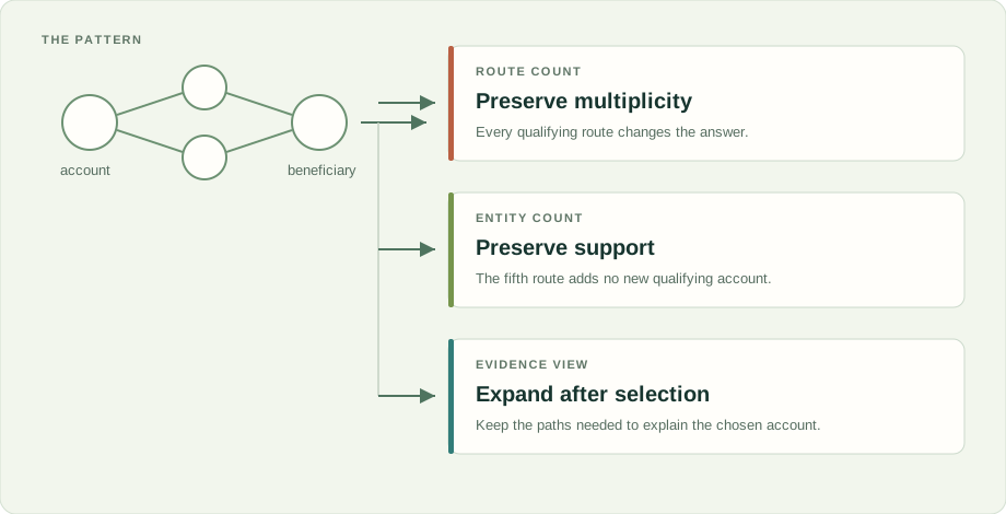
One pattern, three jobs

Suppose an analyst follows an account through intermediaries to sanctioned beneficiaries. Three questions can use the same visual pattern:

• How many transfer routes reach a sanctioned beneficiary?
• How many origin accounts have at least one such route?
• Which routes explain why account 731 entered the review queue?

The first question needs multiplicity. If five routes connect the same endpoints, all five count. The second needs support by origin account; the fifth route adds cost but no new account. The third needs inspectable evidence for one selected candidate. A plan that expands every route is faithful to the first question and extravagant for the second. A plan that keeps only existence is efficient for the second and wrong for the first. An evidence view that returns one arbitrary route can mislead the third.

This difference sounds obvious when written in three bullets. It disappears easily inside a query plan, especially after another branch adds merchant ownership, device use, location, or time. The intermediate rows begin to represent combinations of facts rather than facts. Cardinality rises even when no new entity enters the answer.

A worked fraud case

Take 20,000 customer accounts. Each uses several payment instruments. A popular processor serves a million merchants. The analyst wants customer accounts that share a device with a confirmed fraud account, send funds through a high-risk merchant, and have no established household relationship with the fraud account.

A naïve plan expands customer-to-device matches, joins every device user, expands every merchant route, then subtracts household relationships. One popular device or processor can dominate the intermediate result. More hardware gives the plan more room to describe the popularity of the processor.

The answer needs something narrower. For each customer, establish support for the device condition and the merchant condition while preserving any identity shared by those conditions. Then evaluate the exclusion against the supported candidates. Only the selected accounts need detailed evidence expansion for review. The engine can reduce work early because the query asks for candidate accounts, not a census of every combinatorial witness.

Now change the question to “how many distinct devices connect each account to confirmed fraud?” The support representation must change. An account with one shared device and an account with twenty no longer mean the same thing. Exact optimization does not come from calling all duplicates redundant. It comes from knowing which duplicates the result can observe.

Shared identity is a hard constraint

Suppose the query requires a supplier that holds a safety certification and serves a restricted market. Testing “has a certified supplier” and “has a supplier in the market” as separate booleans can produce a false result: supplier A holds the certificate, supplier B serves the market, and neither satisfies both.

The shared supplier variable is a promise made by the query. The optimizer must keep that identity until it proves both conditions on the same supplier. This is where many attractive shortcuts stop being algebra and become wishful thinking.

The best regression for this rule contains only two suppliers. Put one condition on each. If the company qualifies, the plan is wrong. Tiny hostile graphs expose semantic errors that large benchmark datasets can hide beneath plausible totals.

Negation raises the stakes. “No direct payment to a sanctioned beneficiary” means the engine must establish absence in the relevant domain and snapshot. It cannot treat a missing row from an incomplete branch as proof. Nulls, relationship reuse, direction, and clause boundaries have similar force. They look like language details until one changes an investigation.

Vector search changes the boundary

Consider a research assistant looking for the ten papers most similar to a claim, restricted to papers that independently evaluate the cited method. Taking the nearest ten vectors and filtering by the graph can return three papers. It can also miss a qualifying paper ranked eleventh in the unfiltered population. “Rank, then filter” and “rank within the eligible graph population” are different questions.

Candidate-first search remains useful when the application wants exploration and accepts that boundary. Exact population-constrained ranking needs a plan that joins vector and graph eligibility without losing the ranking contract. ShrikeDB keeps vector results on the same entity identity as graph data so applications can state that boundary directly and inspect the work.

GraphRAG makes the distinction practical. Twenty passages from one survey can consume a context window while contributing one source. A graph-aware retrieval can limit each source, require an evidence relationship, or separate independent evaluations from citations by the original group. The graph earns its cost when it changes the evidence set, not when it decorates a semantic search with arrows.

What to test in your own graph

Choose one expensive production query and build four variations of the data while keeping node and edge totals similar:

• Concentrate many routes through one high-degree entity.
• Add several routes to the same destination.
• Make two branches share a variable, then split their conditions across different entities.
• Add an exclusion edge to a small fraction of otherwise qualifying candidates.

Measure completion coverage and tail latency, then verify the answers independently. Ask the engine for a count, a distinct-entity list, and evidence for selected entities. Their runtime curves should reflect their different information requirements. If all three plans enumerate the same universe, you have found the ceiling before the production graph does.

This is the reason for ShrikeDB. We want complex queries to remain exact when the graph becomes awkward, multimodal, and large. The work should follow the information in the answer rather than the number of combinations available along the way.