02 / Evidence
A relationship is a claim, not a line
The graph makes correlation easy to draw. Good analysis keeps the rule, the evidence, and the alternatives close enough to question.
Two vessels report from the same area within five minutes. Two cards use the same terminal within five minutes. Two machines fail after receiving the same batch. These patterns are excellent candidate generators. They are poor conclusions.
The trouble begins when a row-level join becomes a durable edge with a persuasive name. Ten matching position reports can describe one co-presence episode. A busy public terminal can connect thousands of unrelated cards. A reporting gap can mean a disabled transmitter, a receiver outage, or simply a vessel beyond coverage. The database cannot rescue a relationship whose name asserts more than its evidence.
ShrikeDB supports a more useful rhythm: query observations, derive relationships for the current question, inspect their evidence, and materialize only when the application has a reason to retain them. Cypher can return query-time relationships as rows. SPARQL CONSTRUCT can return a result graph without inserting triples into the source graph.
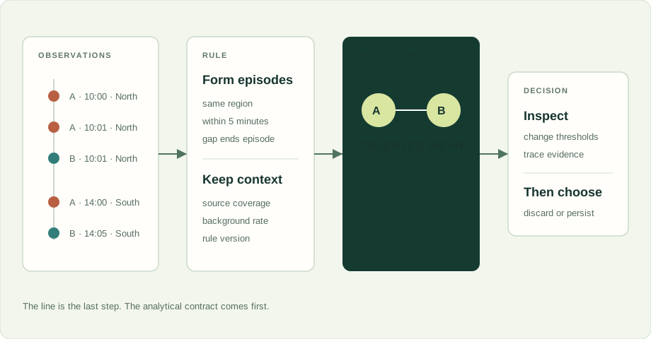
Pairs, episodes, and claims
Start by deciding what one result represents. A matching pair means two observations satisfy a predicate. An episode means a set of observations forms one continuous occurrence under a gap rule. A relationship means the application assigns a durable interpretation to one or more episodes.
Those units are not interchangeable. Improve one sensor from ten-minute reports to one-minute reports and pair counts can rise by an order of magnitude with no change in behavior. Episode counts may remain stable. A model that scores raw pairs can quietly learn sensor policy instead of activity.
The same mistake appears in finance. If two accounts each pay a common processor one hundred times, the join yields ten thousand transaction pairs. That does not describe ten thousand independent associations. It describes two accounts, one common counterparty, and a great deal of repeated evidence whose significance depends on how ordinary that processor is.
A worked movement example
Entity A reports in the North zone at 10:00, 10:01, and 10:02. Entity B reports there at 10:01. Later, A reports in the South zone at 14:00 and B at 14:05.
| Entity | Time | Zone | Source |
|---|---|---|---|
| A | 10:00, 10:01, 10:02 | North | receiver-7 |
| B | 10:01 | North | receiver-7 |
| A | 14:00 | South | receiver-2 |
| B | 14:05 | South | receiver-2 |
An inclusive one-minute rule produces three North observation pairs. A five-minute rule adds one South pair. The result contains four pairs, two qualifying zones, one entity pair, and perhaps two episodes. “Perhaps” matters: episode boundaries require a continuity rule. If a ten-minute gap ends an episode, the North and South facts cannot belong to one occurrence. If source coverage failed between them, even the apparent separation needs context.
A query can legitimately return OBSERVED_NEAR with the observation IDs, interval, region, and thresholds that produced it. It cannot infer communication or intent from proximity alone. Analysts may combine the result with ownership changes, communication records, cargo events, or repeated routes. Each added condition strengthens a question. None turns the original observation into a different fact.
Now move the same reasoning into a fraud graph. Replace zones with merchants and position reports with transactions. “Same merchant within five minutes” may identify coordinated testing of stolen cards, or it may identify the coffee shop outside a railway station at 08:30. The pattern finds candidates. The background tells you whether the pattern is interesting.
The background rate belongs in the graph
A shared counterparty has a degree, a role, a schedule, and a population with an opportunity to use it. Compare entities against an appropriate background before ranking the relationship. Ten shared counterparties can be unusual among small exporters and ordinary among subsidiaries using one treasury service.
This leads to better questions:
- How many unrelated peers use the same resource during the same interval?
- Does the pair recur across independent locations or counterparties?
- Does the behavior survive a tighter time or distance threshold?
- Did collection coverage change when the pattern appeared?
These are graph questions because context sits around the candidate. They are temporal questions because order and recurrence matter. They are statistical questions because searching millions of pairs will produce visually striking coincidences. One score cannot replace those distinctions.
Group behavior needs another precaution. A met B on Monday, B met C on Tuesday, and A met C on Wednesday. The pairwise projection is a triangle. A, B, and C did not necessarily meet as a group. If joint participation matters, keep the event as an entity and connect participants to it. Derive the triangle for display when useful, but retain the event identity that distinguishes one gathering from three separate meetings.
Build a result graph first
A result graph lets an analyst work with derived structure without rewriting history. It can contain candidate relationships, episode nodes, supporting observation IDs, parameters, and the source version used by the query. Two analysts can use different thresholds against the same observations and compare results without deleting each other’s interpretation.
SPARQL CONSTRUCT suits this job because the output is a graph scoped to the query. Cypher can return the same analytical structure as entities, relationships, and evidence rows. ShrikeDB preserves the shared entity IDs, so the client can move from a candidate edge back to graph context, vector similarity, a key–value payload, or the underlying geospatial events.
If the relationship later becomes operational state, materialize it with provenance. Store the rule version, input version, evidence identifiers, and creation time. A late event or corrected identity can then produce a new derivation that the application compares with the old one. An edge that disappears becomes an explainable revision instead of a small mystery living in a dashboard.
A practical analyst workflow
Begin broad enough to find candidates, then strengthen the question in visible steps:
- Find conjunctions. Select entities that satisfy two or more place, time, counterparty, or behavior conditions.
- Form episodes. Group observation pairs under explicit continuity and gap rules.
- Compare context. Measure the resource’s background population and the entity’s ordinary behavior.
- Test stability. Change one threshold and show which relationships persist, appear, or vanish.
- Explain the candidate. Return the events and paths that support the selected result.
- Materialize deliberately. Persist only the relationship states that another workflow must address later.
This workflow gives the interface something useful to visualize: not merely a bright line between two dots, but the observations, episodes, and assumptions behind it. It also travels well. Movement analysis, payment networks, maintenance histories, intelligence records, and cyber telemetry all produce candidate relationships whose meaning changes with time, coverage, and background rate.
The interesting graph is often the one the analyst constructs for today’s question. Keep it close to the evidence until it earns a place in tomorrow’s database.